Better than yesterday

본 논문을 읽고 요약한 내용이며 잘못 해석한 내용이 있을 수 있습니다. 설명에 오류가 있다면 댓글로 알려주시면 감사하겠습니다. 

[Introduction] 

 최근 ViT가 좋은 성능을 보이며 image classification, object detection, semantic segmentation과 같은 다양한 computer vision task에 적용되고 있다. 그러나 여전히 deployment 관점에서 ViT는 CNN에 비해 훨씬 느려 CNN이 지배적이다. 많은 연구에서 ViT의 high frequency 딜레마를 극복하고자 노력하였다. 그러나 대부분의 hybrid 구조들은 단순히 CNN을 쌓은 이후 마지막에 Transformer를 ㅈ거용하는 방식이다. 이러한 구조는 downstream task에서 성능 포화를 불러온다. 더욱이 선행 연구에서 CNN과 Transformer block은 efficiency와 performance를 동시에 만족시키지 못한다는 것을 발견했다. 

 이러한 문제점을 해결하기 위해 저자들은 효율적인 Transformer를 설계하기 위한 세가지 요소 NCB, NTB, NHS를 제안하였다. 

 제안된 구조는 latency-accuracy trade-off에서 가장 우수하다. 

 본 논문의 주요 기여는 다음과 같다. 

- 효과적인 convolution block과 transformer block, i.e. NCB와 NTB를 제안하였다. Next-ViT는 NCB와 NTB를 효과적으로 쌓은 hybrid 구조이다. 

- hybrid 구조를 설계하는 새로운 관점을 제시하였다. 

- 다양한 실험을 통해 Next-ViT의 우수성을 입증하였다. SOTA를 능가하는 성능을 보인다. 

[Methods]

  저자가 제안한 모델의 전체 구조는 Figure 2와 같다. 선행 연구에서 제안된 Hybrid 모델들은 CNN block을 연속적으로 쌓고 그 이후 Transformer block을 쌓는 형태로 설계되었다. 저자는 이러한 Hybrid 구조가 downstream task에서 성능 포화를 가지고 온다고 생각하였다. 따라서 각 스테이지에서 두 가지를 결합한 형태를 사용하였다. 본 논문에서 제안한 Next-ViT는 Next Convolution Block (NCB), Next Transformer Block (NTB)로 구성되어 있으며 Next Hybrid Strategy (NHS)를 통해 탐색되었다. Next-ViT는 hierarchical pyramid architecture를 따라 구성되었다. 전체적인 구조는 Patch Embedding과 각 스테이지의 convolution 혹은 transformer block으로 이어진다. 

Next Convolution Block (NCB)

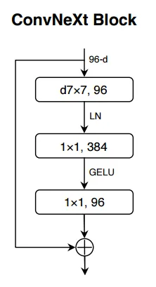
 저자들은 NCB를 제안하기위해 고전적으로 제안되었던 구조들을 검토하였다. Figure 3(a)는 ResNet에서 제안된 BottleNeck block으로 내재된 inductive bias와 deployment-friendly 특성으로 대부분의 하드웨어에서 오랜 기간 사용되었다. 그러나 Transformer block에 비해 부적절하다. ConvNeXt block은 Transformer block의 구조를 모방하여 BotteNeck을 수정한 것으로 성능 향상을 보였으나 TensorRT, CoreML에서 제한적이다. (7x7 depthwise convolution, LayerNorm, GELU) Transformer block은 좋은 성능을 보이지만 attention mechanism의 계산 복잡도로 인해 inference speed는 CNN-based block에 비해 느리다. 

 이러한 점을 극복하여 Transformer block의 성능을 내며 Bottleneck의 배포 측면에서의 장점을 가져가는 Next Convolution Block (NCB)를 제안하였다. NCB는 일반적인 Transformer block의 구조를 차용하되, attention 연산을 줄이기 위해 새로운 Multi-Head Convolutional Attention (MHCA)를 적용하였다. (deployment-friendly) 

 최종적인 NCB의 구조는 MHCA + MLP로 Transformer block의 패러다임을 따른다. 

Multi-Head Convolutional Attenttion (MHCA)

 저자는 attention-based token mixer의 high latency 딜레마를 해결하기 위해, 효율적인 Convolutional Attention (CA)를 활용한 어텐션 메커니즘을 제안하였다. 

 효과적인 local representation learning을 위해 MHSA와 마찬가지로 다중 헤드 패러다임을 사용하였다. 

MHCA는 h개의 하위공간의 정보를 캡처한다. z = [z1, z2, ...,zh]는 input feature z를 채널 차원에서 multi-head form으로 나누는 것을 의미한다. 다중헤드 사이의 정보 상호작용을 촉진하기 위해, projection layer (W)를 장착한다. 

 CA는 single-head convolutional attention으로 위의 식과 같이 인접한 토큰과 trainable parameter W의 내적으로 정의된다. CA는 local receptive field에서 trainable parameter W를 반복적으로 최적화하여 다른 토큰 사이에서 유연하게 학습할 수 있다. 

 정확한 구조는 Figure 4와 같다. MHCA는 group convolution (multi-head convolution)과 point-wise convolution (conv 1x1)로 구성된다. TensorRT의 다양한 데이터 타입에서 빠른 inference를 위해 head dim은 32로 설정하였다. 

 추가적으로, 빠른 추론속도를 위해 전통적인 구조에서 사용하는 LN과 GELU대신 BN과 ReLU를 사용하였다. 

Next Transformer Block (NTB)

 Transformer block은 global 정보를 담고있는 low-frequency signla을 잘 캡처하는 특징을 가지고 있다. 그러나 Figure 5에서 볼 수 있듯 high-frequency 정보는 담지 못한다. 실제 인간의 시각 시스템에서 서로 다른 주파수의 신호는 정확한 특징 추출을 위해 융합하여 사용된다. 

 이러한 관찰에 영감을 얻어 다양한 주파수의 신호를 감지하면서 경량화된 Next Transformer Block (NTB)를 제안하였다. 

 제안된 구조는 Figure 6과 같다. NTB는 먼저 E-MHSA를 통해 low-frequency signal을 캡처한다. 

식으로 나타내면 위와 같다. SA는 Linear SRA에서 차용한 spatial reduction이다.

P_s는 공간차원을 downsampling하기 위한 것으로 stride를 s로 한 avg-pool 연산을 의미한다. attention 연산 전에 avg-pooling을 적용하여 연산량을 줄이고자 하였다. 저자들은 E-MHSA의 시간 소비가 채널 수에 큰 영향을 받는다는 것을 관찰하였다. 따라서 attention 전에 conv 1x1을 진행하여 채널 차원을 줄이고 inference를 가속화하고자 하였다. r은 channel reduction을 의미한다. 

 이후, multi-frequency signal을 캡처하기 위해 MHCA 모듈을 적용시켰다. 이러한 구조는 high-low frequency의 정보를 융합할 수 있도록 한다. 마지막으로 MLP layer를 붙였다. 여기서도 NCB에서와 마찬가지로 LN과 GELU 대신 BN과 ReLU를 적용하였다. 

Next Hybrid Strategy (NHS)

 선행 연구들은 CNN과 Transformer를 결합한 구조가 배포에 효과적임을 보여준다. 

 Figure 7(b)(c)를 보면 대부분의 선행 연구에서 각 스테이지에서는 CNN, Transformer만을 사용하고 마지막 스테이지에서만 Transformer를 쌓는 방식으로 설계되었음을 알 수 있다. 하지만, 이러한 방식은 downstream task에서 효과적이지 않다. classification은 단순히 마지막 output을 사용해 예측을 진행하지만 segmentation, object detection과 같은 downstream task의 경우 각 스테이지에서 어떤 feature를 추출하는지에 따라 성능이 결정되기 때문이다. 

 따라서 저자들은 NCB와 NTB를 (N+1) * L 패러다임으로 쌓는 Next Hybrid Strategy (NHS)를 제안하였다. 먼저, 각 스테이지에서 global information을 캡처할 수 있게 하기 위해 (NCB x N + NTB x 1) 패턴으로 설계하였다. 특히 NTB block은 각 스테이지에서 global representation을 학습하기 위해 스테이지에 마지막에 배치되었다. 

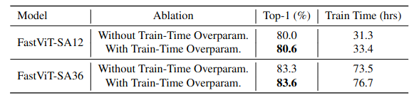
어떤 구조가 효과적인지 알아보기 위해 여러가지 조합에 대한 실험을 진행하였다. C는 한 스테이지가 모두 convolution block으로 구성된 것, T는 한 스테이지가 모두 Transformer block으로 구성된 것, H_N은 NHS로 설계된 것을 의미한다. 공정한 비교를 위해 TensorRT latency가 비슷할 때 downstream task에서의 정확도를 비교하였다. Table 1을 보면 CHHH로 설계했을 때 가장 좋은 성능을 보였다. 

 또한 큰 모델에서도 이러한 구조가 효과적인지 알아보기 위해 실험을 진행하였다. 

우선 Table 2의 윗부분을 보면 N의 개수를 늘려 크기를 조정했을 때 성능 포화에 달성한 것을 볼 수 있다. 이는 N을 늘려 크기를 늘리는 것은 좋은 방법이 아님을 의미한다. 따라서 (NCB X N + NTB X 1) 패턴을 유지하고 이를 여러번 쌓는 방식으로 크기를 늘려 성능을 비교하였다. 그 결과 이러한 패턴이 더 좋은 성능을 나타냈다. 이는 이러한 패턴이 다양한 주파수의 신호를 조합하는 것이 좋은 질의 representation learning으로 이어짐을 의미한다. Table 2에서 N=4일 때 performance-latency trade-off가 가장 우수했다. 

 식으로 나타내면 위와 같다. 

Next-ViT Architectures 

 SOTA와의 공정한 비교를 위해 S/B/L 크기로 모델을 설계하였다. C는 output channel, S는 각 스테이지의 stride를 의미한다. 또한 r은 0.75, s는 [8, 4, 2, 1]로 사용하였다. 

[Experiments]

ImageNet-1K Classification 

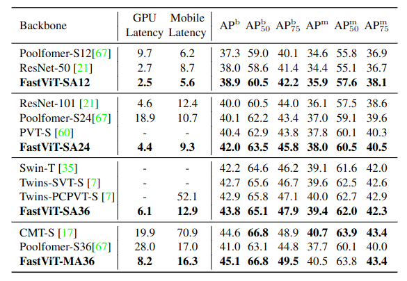
 ImageNet-1k dataset에서 모델 크기에 따라 다양한 SOTA 모델과 performance-latency trade-off를 비교하였다. 

Next-ViT-S와 CMT-XS, Twins-SVT-S, ResNet101 모델과 비교한 결과 더 빠른 속도를 내면서 더 좋은 성능을 나타냈다. 여기서도 볼 수 있듯이 파라미터와 FLOPs가 더 많더라도 latency가 더 빠를 수 있다. 

ADE20K Semantic Segmentation 

 Detection과 segmentation task에서 Mask R-CNN과 Upernet의 일부 모듈로 인해 TensorRT와 CoreML로 변환하는 것이 쉽지 않아 공정한 비교를 위해 backbone latency만을 측정해 비교하였다. latency 측정에서는 input size를 512 x 512로 사용하였다. 

Object Detection and Instance Segmentation 

Ablation Study and Visulaization

Next-ViT를 더 잘 이해하기 위해 Fourier spectrum과 heatmap을 사용해 분석하였다. 

Impact of Next Convolution Block 

NCB의 효과를 입증하기 위해 NCB를 다른 block으로 대체하여 실험을 진행하였다. 공정한 비교를 위해 TensorRT latency를 비슷하게 유지하였다. Table 7을 보면 NCB가 가장 우수한 성능을 보임을 알 수 있다. 

Impact of Different Shrink Ratios in NTB 

또한 shrink ratio r의 영향을 알아보기 위해 실험을 진행하였다. Table 8을 보면 r이 작아질수록 latency가 줄어듬을 알 수 있다. 또한 r이 0.5, 0.75일 때 r=1일때보다 더 좋은 성능을 보였다. 이는 multi-frequency를 융합한 것이 더 좋은 성능을 낸다. (r은 E-MHSA 모듈의 채널 수로, r=1일때는 pure transformer를 의미한다. 저주파만 감지하는) 

Impact of Normalization and Activation 

 서로 다른 normalization layer와 activation function의 영향에 대한 실험도 진행하였다. LN과 GELU를 같이 사용하는 것이 더 좋은 성능을 냈으나 높은 latency를 보였다. 반면, BN과 ReLU는 가장 좋은 latency/accuracy trade-off를 보였다. 

Visualization 

 Next-ViT의 표현능력을 보기 위해 Fourier spectrum, heat map을 이용해 output feature를 시각화하였다. Figure 5(a)를 보면 ResNet은 high-frequency, Swin은 low-frequency만을 캡처하는 것을 볼 수 있다. 반면 Next-ViT는 두 신호를 잘 표현하고 있다. 또한 Figure 5(b)를 보면 Next-ViT가 global한 정보를 더 잘 캡처하는 것을 볼 수 있다. 

[Conclusion] 

 본 논문에서는 mobile device와 server GPU를 위한 효과적인 구조 Next-ViT를 제안하였다. 실험을 통해 Next-ViT가 SOTA에 비해 latency/accuracy trade-off가 우수함을 입증하였다. 본 논문은 visual neural network에서 학문적 연구와 industrial deployment를 이어주는 역할을 했다는 데 의의가 있다. 

본 논문을 읽고 요약한 내용이며 잘못 해석한 내용이 있을 수 있습니다. 설명에 오류가 있다면 댓글로 알려주시면 감사하겠습니다. 

[Abstract]

 Semantic segmentation은 robotics, 특히 autonomous driving에서 중요한 모듈이다. 대부분의 semantic segmentation는 computationally efficient solution이 아닌 accuracy를 향상시키는데 초점을 맞추었다. 대부분의 efficient semantic semgentation algorithm은 확장성 없이 개별로 맞추어 최적화되었고, 그들을 비교할만한 방법도 없다. 본 논문에서는 real-time segmentation benchmarking framework를 제시하고 자율주행을 위한 다양한 sementation 알고리즘에 대해 연구한다. 또한, generic meta-architecture을 구현하였다.

[Motivation]

 자율주행과 같은 task에 적용하기 위해 computational efficiency는 중요한 역할을 함에도 불구하고 이전까지 Semantic segmentation 모델의 접근은 accuracy나 robustness에 초점을 맞추었다. 몇몇 연구가 efficient 모델 설계를 제안하기는 했으나, 다른 네트워크 혹은 meta-architecutres 사이의 비교 기준이 아직 없다. 이전 연구들은 전체적인 모델 비교만 있을뿐,  다른 module의 영향을 비교하지 않았다. 이러한 접근으로 연구자들은 필요한 task에 맞는 적절한 design choice를 하기 어렵다. 

 본 논문에서는 real-time segmentation을 위한 framework를 처음으로 제안한다. 주요 contribution은 아래와 같다. 

(1) we provide a modular decoupling of the segmentation architecture into feature extraction and decoding method which is termed as meta-architecture as shown in Figure 1. 

(2) A detailed ablation study highlighting the trade-off between accuracy and computational efficiency is presented. 

(3) The modular design of our framework allowed the emergence of two novel segmentation architectures using MobileNet and ShuffleNet with multiple decoding methods. 

[Methodology]

 실험 세팅은 본 논문 참고. 따로 정리할 만한 내용 없음. 

SkipNet-ShuffleNet은 Jetson TX2에 배포하여 image resolution 640 x 360에서 초당 15 frame의 real-time 성능을 달성했다. 

[Datasets]

train : encoder trained on ImageNet

test : Cityscapes (5000 images with fine annotation, with 20 classes including the ignored class. Another section of the dataset contains coarse annotation with 20,000 labeled images.) (resolution : 512 x 1024)

[Result]

 본 논문에서 제시한 framework는 연구자들이 새로운 encoder와 decoder를 시스템적으로 평가하는 방식을 제시하였다. 새로운 computationally efficient model은 GFLOPs에서 SOTA를 달성했다. Jetson TX2에서 ~16 fps의 real-time을 달성했다. 

[Limitation]

 Test 방식은 GPU에서 GFLOPs를 줄이고 embedded에 적용하는 방식으로 사용되었다. 구조적 효율성을 FLOPs/ 파라미터 등으로 평가하였다. 고정된 이미지 해상도에 대해서만 평가되었다. 초당 fps, 시간만 측정되었고 JetsonTX2에서의 정확도 측면에서는 평가되지 못했다.

본 논문을 읽고 요약한 내용이며 잘못 해석한 내용이 있을 수 있습니다. 설명에 오류가 있다면 댓글로 알려주시면 감사하겠습니다. 

[Abstract]

 본 논문의 저자는 latency-accuracy trade-off에서 SOTA를 달성하고 있는 hybrid vision transformer architecture인 FastViT를 소개하였다. 끝으로는 FastViT를 이루고 있는 block 중 하나인 RepMixer라고 불리는 novel token mixing operator를 소개하였다. RepMixer는 네트워크에서 skip-connection을 제거함으로써 메모리 접근 비용을 줄이기 위해 structural reparameterization을 사용하였다. 또한 train time overparametrization과 accuracy를 높이기 위해 large kernel convolution을 적용하였고, 실험적으로 이러한 선택이 latency를 줄이는 데 효과가 있음을 입증하였다. 기존의 모델과 비교했을 때 ImageNet dataset에서 같은 정확도를 달성하면서 더 빠른 속도를 보여준다. 또한 image classification, detection, segmentation, 3D mesh regression과 같은 다양한 task에서 mobile, desktop GPU 모두에서 유의미한 latency 개선을 보여준다.

[Motivation]
 효율적인 네트워크를 설계하면서 높은 정확도를 설계하기 위해 Convolution과 transformer구조를 병합하는 하이브리드 방식이 주로 등장하고 있다.최근 공개된 Metaformer 구조는 skip connection이 있는 token mixer와 다른 skip connection이 있는 FFN으로 구성되는데, 이러한 skip connection 구조는 메모리 액세스 비용이 발생해 상당한 오버헤드를 발생시킨다. 따라서 본 논문에서는 이러한 구조적인 오버헤드를 Reparametrization 기법으로 해결하고자 하였다.

[Methodology]

Reparameterizing Skip Connections

RepMixer

Convolutional mixing은 ConvMixer에서 처음으로 소개되었다.

(ConvMixer는 ViT의 성능이 transformer 아키텍처로 인한 것인지, 아니면 input representation으로 patch를 사용한 것이 영향을 끼쳤는지에 대해 탐색하는 논문. patch embedding layer 이후 반복되는 단순한 convolutional block으로 구성된 간단한 구조)

ConvMixer Layer는 위의 그림에서 보이는 것과 같이 input tesor를 X라고 할때,

Y = BN(\sigma(DWConv(X)) + X로 구성되어 있다.

여기서 sigma는 non-linear activation (그림에서는 GELU), DWConv은 depthwise convolutional layer를 의미한다. 이러한 block이 RepMixer에서 효과적이기 때문에 간단히 연산을 rearrange하고, non-linear activation을 제거하여 

Y = DWConv(BN(X) + X 와 같이 식을 구성하였다. 이렇게 디자인한 이유는 Inference시 Figure 2d 와 같이 Y=DWConv(X)로 바뀔 수 있기 때문이다.

Positional Encoding

저자들은 동적으로 생성되고 input token의 local neighborhood에서 동작하는 conditional positional encoding을 사용하였다. 이러한 encoding은 depth-wise convolution operator의 결과로 생성되고 patch embedding에 추가된다.이 작업에서는 non-linearity가 없어 reparametrized될 수 있다.

Linear Train-time Overparameterization

Efficiency를 더욱 증가시키기 위해, 모든 dense k x k conolution을 그것의 factorized version으로 대체하였다. 즉, k x k depthwise follwed by 1 x 1 pointwise convolution 으로 대체하였다. 그러나 factorization으로 인한 적은 parameter수는 model의 capacity를 감소시킬 수 있다. 이를 증가시키기 위해 MobileOne에서 소개된 linear train-time overparameterization을 사용하였다. 

그러나 train-time overparamaterization은 추가된 분기의 오버헤드로 trainig time이 증가하는 결과를 보인다. 따라서, dense k x k convolution with factorization 부분만 대체하였다. (이러한 layer는 convolutional stem, patch embedding, projection layer에서 발견되나 일부만 선택하여 대체)

Large Kernel Convolutions

RepMixer의 receptive field는 self-attention token mixer에 비해 local이다. 그러나, self-attention 기반의 token mixer는 계산량이 매우 많다. self-attention을 사용하지 않는 초기 stage에서 receptive field를 효율적으로 개선하는 방법은 deptwise large kernel convolution을 통합하는 것이다. 따라서 FFN 및 patch embedding layer에 depthwise convolution을 도입한다.

Table 4의 V3와 V5를 비교해보면, V3가 V5에 비해 0.4%의 작은 정확도 증가를 보이면서 모델 사이즈가 11.2% 크고, latency가 2.3배 높은 것을 볼 수 있다. V2와 v4를 비교해봐도 얻는 accuracy에 비해 standard setting이 효율적이지 못한 것을 알 수 있다.

Table 1의 LK.conv.FFN과 LK.conv.Patch Emb. 결과를 보면 전체적으로 large kernerl convolution이 정확도 개선을 보인 것을 알 수 있다.

 FFN과 patch embedding layer의 구조는 Figure 2와 같다. FFN block은 ConvNeXt block과 비슷하나 몇 가지 차이가 있다.

ConvNeXt Block에서 LN을 사용하는 것과 반대로 BN을 사용한다. 이는 이전 레이어와 융합될수 있기 때문이다. 또한 LN을 사용할 떄는 적절한 tensor layout을 얻기위해 적절한 변형 작업이 필요하다. 그러나 이렇게 대체하면 추가적인 reshape operation이 필요하지 않다.

[Datasets]

Image Classification : ImageNet-1K

Robustness Evaluation : ImageNet-A, ImageNet-R, ImageNet-Sketch, ImageNet-C

3D Hand mesh estimation : FreiHAND

Semantic Segmentation : ADE20k

Object Detection : MS-COCO

[Result]

Image Classification

Robustness Evaluation

3D Hand mesh estimation

Semantic Segmentation and Object Detection

[Limitation]

[Idea]

본 논문을 읽고 요약한 내용이며 잘못 해석한 내용이 있을 수 있습니다. 설명에 오류가 있다면 댓글로 알려주시면 감사하겠습니다. 

[Abstract]

 Vision Transformer는 vision task에서 진전을 보이고 있고, 다양한 benchmark에서 유의미한 결과를 얻었다. 그러나 파라미터 수가 많고 attention mechanism과 같이 2차 복잡도를 지니는 구조적인 한계 때문에 경량화된 CNN보다 몇 배는 더 느리다는 단점이 있다. 따라서 실제 어플리케이션에 배포하는게 힘들고, 특히 모바일 디바이스와 같이 제약된 하드웨어에서 이러한 단점이 부각된다.

본 논문의 핵심 질문은 'can transformers run as fast as MobileNet while obtaining high performance?'이다. 이를 위해 본 논문에서는 ViT 기반 모델의 디자인 구조를 다시 살펴보고 새로운 구조를 제안하고자 한다.

[Methodoloy]

On-Device Latency Analysis of Vision Transformers

대부분의 접근 방식은 GPU에서 얻을 수 있는 computation complexity (MACs) 또는 throughput (images/sec)을 통해 transformer의 inference 속도를 최적화하는 것이다. 그러나 이러한 metric은 실제 on-device latency를 반영하지 않는다. Edge device에서 ViT의 속도를 늦추는 원인이 무엇인지 파악하기 위하여 Figure1과 같이 다양한 모델에 대해 latency analysis를 진행하였다.

Observation 1: Path embedding with large kernel and stride is a speed bottleneck on mobile deivces.

Patch embedding은 kernel size와 stride가 큰 non-overlapping convolution layer로 구현되는 경우가 많다. (Figure 2의 모습처럼 겹치지 않게 하기 위해 kernel, stride 사이즈를 16등 크게 설정)

일반적으로 transformer에서 patch embedding layer의 계산 비용이 크지 않다고 생각되어져왔다. 그러나 Figure 1의 DeiT-S 및 PoolFormer-S24(Large kernel & stride)와 LeViT-256을 보면 큰 차이가 있다는 것을 알 수 있다. Large-kernel convolution은 대부분의 컴파일러에서 잘 지원되지 않으며, 가속화될 수 없는 부분이기 때문이다.

*) Reference https://engineering.linecorp.com/ko/blog/neural-network-on-mobile-gpu

TF Lite에서 3x3 필터를 사용하는 합성곱 연산이 Winograd 합성곱 알고리즘(행렬곱 기반의 합성곱보다 수행해야 할 곱셈 연산을 줄여줌)의 가속을 받아 성능이 크게 향상됨.

따라서 저자는 kernel, stride 대신 3x3 사이즈의 kernel을 가지는 CNN + fast downsampling조합으로 Patch embedding을 구현하였다. (Figure 3의 CONV stem)

Observation 2 : Consistent feature dimension is important for the choice of token mixer. MSA is not necessarily a speeed bottleneck.

(LeViT와 PoolFormer 비교) LeViT-256의 대부분은 4D tensor의 CONV으로 구현되며, 패치된 3D tensor에서 attention을 수행해야 하기 때문에 feature를 MSA로 전달할 때  reshape 과정이 여러 번 수행된다. 이렇듯 Reshape를 광범위하게 사용하면, 모바일 장치에서의 LeViT 속도가 제한된다. 반면, Pooling은 4D tensor에 적합하다.

(LeViT와 DeiT 비교) feautre dimension이 일관되고, Reshape가 필요하지 않은 경우 MSA가 오버헤드를 가져오지 않는다.

( 구조적인 차이점을 분석하여 내린 결론 )

 따라서 위의 관찰 결과를 바탕으로 저자는 4D feature implementation과 3D MSA를 가지고 비효율적인 빈번한 reshape를 제거하는  dimension-consistnet network를 제안하였다.

Observation 3 : CONV-BN is more latency-favorable than LN (GN)-Linear and the accuracy drawback is generally acceptable.

MLP block은 보통 LN+3D linear projection과 CONV 1x1+BN(Batch Norm) 중 하나가 선택된다. Figure 1을 보면, LN이 network inference time 중 10~20% 정도를 차지하는 것을 볼 수 있다. LN과 같은  dynamic normalization은 inference 단계에서 실행 중인 statistics를 수집하여 latency에 기여한다. 반면, Conv-BN구조는 4D tensor에 대해 연산을 하고 inference 할 때, BN이 Conv 구조에 folding될 수 있으므로 latency를 낮추는 데 더 용이하다. 하지만, Conv-BN은 LN에 비해 성능이 조금 낮게 나온다.

따라서 저자는 token mixer가 pooling일 때는 Conv-BN을 사용하고,  MSA일 경우 LN-Linear를 사용하였다. (원래 ViT설계와 일치하게 하기 위해)

Observation 4 : The latency of nonlinearity is hardware and compiler dependent.

GeLU, ReLU, HardSwish와 같은 activation에 대해서도 조사하였다. 선행 연구에서 GeLU가 hardware에 효율적이지 않다고 알려져있으나, iPhone 12에서는 오히려 ReLU보다 GeLU가 더 적합한 것으로 나타났다. (LeViT-256 latency with HardSwish is 44.5 ms while with GeLU 11.9 ms) 따라서 EfficientFormer에서는 GeLU를 사용한다.

Design of EfficientFormer

EfficientFormer는 patch embedding(CONV stem)과 여러 개로 쌓은 meta block(MB)로 구성된다. MB 3D는 transformer기반, MB 4D는 CNN을 기반으로 만들어졌다.  각 단계 사이에는 Embedding으로 표시된 임베딩 차원과 downsample token lenght를 투영하는 임베딩 작업이 있다. 각 Stage는 여러 개의 MB로 구성되어있고 같은 stage내에서는 같은 spatial size를 가진다.

Latency Driven Slimming

Design of Supernet.

dimension-consistent design을 위해 supernet으로부터 NAS를 사용해 최적 구조를 찾는다. Supernet은 위와 같은 MetaPath(MP)를 정의하여 구성된다. MB 3D는 마지막 두 개의 stage에서만 가능하도록 하였다.

이렇게 설계한 이유는 첫째, MSA의 계산은 token length에 quadratic하게 증가하기 때문에 앞쪽에 두게 되면 계산이 너무 증가하게 된다. 두 번째로 global MSA를 뒤쪽에 놓는 것은 앞쪽에서는 low-level feature를 뒤쪽 layer에서는 long-term dependency를 capture한다는 직관과 일치하기 때문이다.

Searching Space. searching space는 각 Stage의 width(C), 각 stage의 block 수 (N), MB 3D에 적용할 마지막 block 이다.

Search algorithm.

supernet의 학습이 완료되면 바로 어떤 path가 best인지 알 수 있는 efficient한 gradient-based search algorithm을 제안한다.

먼저, supernet training 씨에 Gumble Softmax sampling을 함께 사용해 선택된 MP의 importance score를 측정한다. 그 다음 16배수로 나누어진 channel(width)들을 가지는 여럿 MB 4D, MB 3D의 on-deivce latency lookup table을 구축한다. 그리고 single-width를 가지는 Supernet 기준으로 채널 수를 조절하는 gradual slimming을 진행한다.

[Result]

EfficientFormer는 PyTorch 1.11과 Timm library를 사용해 구현되었다. 모델은 NVIDIA A 100, V 100 GPUs에서 학습되었다. mobile speed는 A 14 bionic chip이 장착되고 NPU 사용이 가능한 iPhone 12에서 1000번 inference하고 평균을 내어 결과를 냈다.

[Conclusion & Limitations]

기존의 모델들에 비해 모바일 환경에서 더 낮은 latency를 달성하면서 성능도 acceptable한 결과를 나타냈다. 그러나 여전히 MobileViT와 같은 모델에 비해 큰 파라미터를 나타낸다. 또한, general-purposed하게 디자인되었지만, GeLU와 같이 플랫폼과의 호환성으로 인해 다른 플랫폼에서는 다른 경향을 띈다.